Appendix 2 - Measuring Electrode Impedance

The measuring of impedance in the ADS1299 is made it by injecting a 6nA altern current at 31.2 Hz, in this example will be measured the impedande in the N inputs (like used for single reference EEG montages), and will be use the leadoff_impedance method to set these inputs in the correct mode.

The first step is to connect correctly the Cyton board to replicate this experiment, a 10K potentiometer will be connected between the N input (bottom) of channel 1 and the SRB2 (bottom), the BIAS pin will not be used in this guide, if you want to test with your head instead of a potentiometer then you must use this pin.

Note

• The impedance measurement does not work correctly on the current version of Cyton Library, but there is a pull request that solve this issue.

• Is possible to use versions between V3.0.0 and V3.1.2, but you must reset the board every time before measurement and NEVER change the sample frequency.

Offline measurement

# openbci = Cyton('serial', '/dev/ttyUSB1', capture_stream=True, daisy=False)
openbci = Cyton('wifi', '192.168.1.113', host='192.168.1.1', capture_stream=True, daisy=False)

openbci.command(cons.SAMPLE_RATE_250SPS)
openbci.command(cons.DEFAULT_CHANNELS_SETTINGS)
openbci.leadoff_impedance(range(1, 9), pchan=cons.TEST_SIGNAL_NOT_APPLIED, nchan=cons.TEST_SIGNAL_APPLIED)

openbci.stream(7)
data_raw = np.array(openbci.eeg_time_series)

show([data_raw[0]])

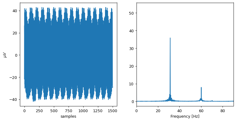
We still not see a sinusoidal at 31.2 Hz but there is one, so, with a filter:

band_2737 = GenericButterBand(27, 37, fs=250)

def filter_impedance(v):
    v = notch60(v, fs=250)
    return band_2737(v, fs=250)

data = filter_impedance(data_raw)
# data = data[:, 100:-100]

show([data[0]])

INFO:root:Compiled `Butter` filter (27|37 Hz) for 250.00 Hz

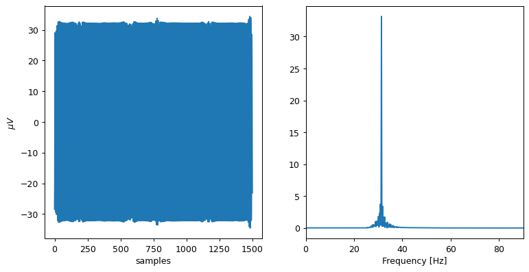
Now we need the RMS voltage, there is a lot of formulas to get this value, even using the std, but I like to use one based on the VPP:

\[V_{RMS}=\frac{V_{pp}}{2\sqrt{2}}\sim std(V)\]

Our Vpp can be calculated as the maximun - minimum. In some approaches, is very common to found the usage of standard deviation instead of RMS.

def get_rms(v):
    return np.std(v)
#     return (v.max()-v.min())/(2*np.sqrt(2))

rms = get_rms(data[0])
rms

24.359166882658073

\[Z=\frac{V_{RMS}}{I_{RMS}}\]

We know that the ADS1299 injects a 6nA of alternating current, so:

\[I_{RMS}=\frac{6nA}{\sqrt{2}}\]

Then, considering that we have uV instaead of V:

\[Z=\frac{\mu V_{RMS}\cdot10^{-6}\cdot\sqrt{2}}{6\cdot10^{-9}}\]

def get_z(v):
    rms = get_rms(v)
    return 1e-6 * rms * np.sqrt(2) / 6e-9

z = get_z(data[0])
print(f'For {rms:.2f} uVrms the electrode impedance is {z/1000:.2f} KOhm')

For 24.36 uVrms the electrode impedance is 5.74 KOhm

The Cyton board has a 2.2K Ohm resistors in series with each electrode, so we must remove this value in way to get the real one.

def get_z(v):
    rms = get_rms(v)
    z = (1e-6 * rms * np.sqrt(2) / 6e-9) - 2200
    if z < 0:
        return 0
    return z

z = get_z(data[0])
print(f'For {rms:.2f} uVrms the electrode-to-head impedance is {(z)/1000:.2f} KOhm')

For 24.36 uVrms the electrode-to-head impedance is 3.54 KOhm

Real time measurement

For this experiment we will use the Kafka consumer interface, and the same potentiometer. Keep in mind that this measurement uses 1 second signal, so, the variance will affect the real measure, in real-life the amplitude not change so drastically.

import time
Z = []
with OpenBCIConsumer('wifi', '192.168.1.113', host='192.168.1.1', auto_start=False, streaming_package_size=250, daisy=False) as (stream, openbci):
# with OpenBCIConsumer(host='192.168.1.1') as stream:

    openbci.command(cons.SAMPLE_RATE_250SPS)
    openbci.command(cons.DEFAULT_CHANNELS_SETTINGS)
    openbci.leadoff_impedance(range(1, 9), pchan=cons.TEST_SIGNAL_NOT_APPLIED, nchan=cons.TEST_SIGNAL_APPLIED)
    time.sleep(1)
    openbci.start_stream()

    for i, message in enumerate(stream):
        if message.topic == 'eeg':

            eeg, aux = message.value['data']
            eeg = filter_impedance(eeg)
#             eeg = eeg[:, 100:-100]
            z = get_z(eeg[0])
            Z.append(z)
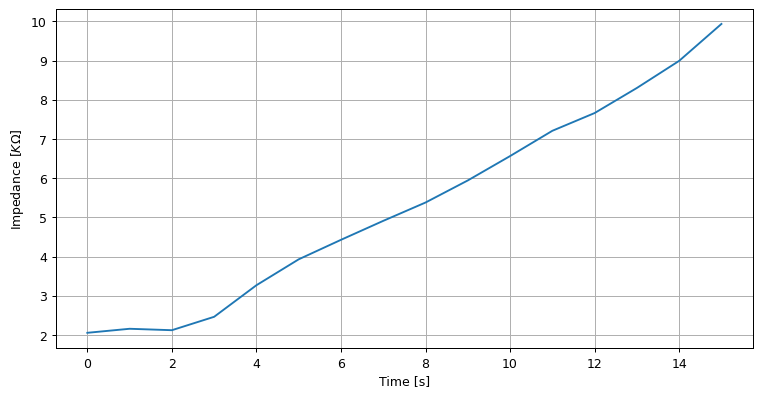
            print(f'{z/1000:.2f} kOhm')

        if i >= 15:
            break

2.06 kOhm
2.16 kOhm
2.12 kOhm
2.46 kOhm
3.27 kOhm
3.93 kOhm
4.43 kOhm
4.91 kOhm
5.38 kOhm
5.94 kOhm
6.56 kOhm
7.21 kOhm
7.66 kOhm
8.30 kOhm
8.99 kOhm
9.94 kOhm

plt.figure(figsize=(10, 5), dpi=90)
plt.plot(np.array(Z)/1000)
plt.ylabel('Impedance [$K\Omega$]')
plt.xlabel('Time [s]')
plt.grid(True)
plt.show()

Improve measurements

Some tips for improving the impedance measurement:

• Take shorts signals but enough, 1 second is fine.

• Remove the first and last segments of the filtered signal.

• Nonstationary signals will produce wrong measurements.

• A single measurement is not enough, is recommended to work with trends instead.